[Reading] Bayesian Personalized Ranking from Implicit Feedback

30 Jun 2021

A new category, “Reading” is introduced, in which I would read and rewrite what I understand in a research paper. And today, I’ll summarize BPR: Bayesian Personalized Ranking from Implicit Feedback [1].

Personalized Ranking System

The personalized ranking system is a ranked list of recommended items for a customer. The interesting point of personalized ranking is to revolve around positive examples (user has interacted with items, e.g: user bought items in the past), negative examples (the user has not interacted with the items, e.g: the user has not bought an item yet) - a mixture of negative feedback (the user is not interested in buying the item) and missing values (the user might buy the items in the future).

Personalized Ranking System
1. Introduction
2. Problem Formulation
3. Bayesian Personalized Ranking (BPR)
4. Implmentation
References

1. Introduction

Recommender systems are a widely applicable problem in industry such as music recommendation, movie/video recommendation, point-of-interest (POI) recommendation and so on. The goal of recommender systems is to provide relevant items based on historical data of users who interacted with them.

In general, most recent works in recommender system focus on two scenarios:

Explicit feedback: user provides explicit feedback, like rating.
Implicit feedback: user clicks/purchases/views times (interacts with).

For explicit feedback, not all systems can get explicit user data while implicit feedback is easy to collect because we can track automatically user interactions. In the real world, implicit feedback is already available in almost any information system – e.g. web servers record any page access in log files.

In the implicit scenario, only positive classes are observed. Researchers used binary values to represent the implicit feedback, 1 means positive (observed), while 0 means negative (non-observed). In the other words, if there exists an interaction between user and item, they are labeled a positive (1), and the others are labeled as negative (0).

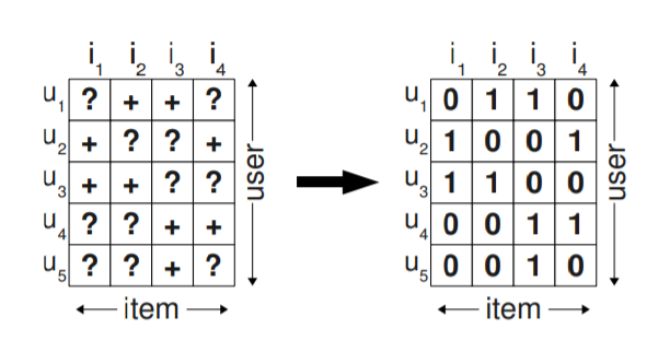
Figure 1. On the left side, the observed data S is shown. Learning directly from S is not feasible as only positive feedback is observed. Usually negative data is generated by filling the matrix with 0 values [1]

However, as mentioned above, the negative cases (non-observed) are a mixture of negative feedback (not interested in) and missing values (potential buyers). Thus, this approach will not take into account ranking recommendation in the future.

In this paper, Rendle et al. propose a (BPR) different way to represent the implicit feedback by using item pairs as training data and optimize the rank list using Bayesian probability.

If you are not more interested in math, you can move on Implementation.

2. Problem Formulation

Let \(U\) and \(I\) be the set of all users and the set of all items respectively. \(S \subseteq U \times I\) is the set of implicit feedback (left side of Fig 1).

The task of the recommender system is now to provide the user with a personalized total ranking \(>_u \subset I^2\) of all items, where \(>u\) has to meet the properties of a total order:

Totality: item \(i\) is preferred over item \(j\), or item \(j\) is preferred over item \(i\):
\[\forall i,j \in I : i \neq j \Rightarrow i >_u j \lor j >_u i\]
Antisymmetry: item \(i\) is preferred over item \(j\), and item \(j\) is preferred over item \(i\) if and only if both \(i\) and \(j\) are the same:
\[\forall i,j \in I : i >_u j \land j >_u i \Rightarrow i = j\]
Transitivity: if item \(i\) is preferred over item \(j\) and item \(j\) is preferred over item \(k\), then the user \(u\) prefers item \(i\) over \(k\):
\[\forall i,j,k \in I : i >_u j \land j >_u k \Rightarrow i >_u k\]

For convenience we also define:

\[I_u^{+} := \{ i \in I : (u,i) \in S \}\] \[U_i^{+} := \{ u \in I : (u,i) \in S \}\]

Where \(I_u^{+}\) is set of all items which user \(u\) interacted with. \(U_i^{+}\) is set of user has interacted with item \(i\).

Training data is formalized as follows:

\[D_S = \{(u,i,j) | i \in I_u^+ \land j \in I \setminus I_u^+\}\]

\(D_S\) is a set of many triples \((u,i,j)\). The sematics of \((u,i,j) \in D_S\) is that user \(u\) is assummed to prefer \(i\) over \(j\).

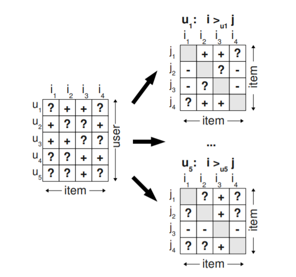
Figure 2.Training data for BPR [1]

In the Fig 2, positive sign shows that a user \(u\) prefers item \(i\) over item \(j\). On contrary, negative sign indicates that \(u\) prefers \(j\) over \(i\). For pairs of items that have both been interacted by a user, we can not infer any preference and marked as ‘?’.

3. Bayesian Personalized Ranking (BPR)

3.1. BPR Optimization

Let \(\Theta\) be the parameter of model. The goal is to maximize posterior probability .

\[\begin{align}p(\Theta | i >_u j) \propto p(i >_u j |\Theta) p(\Theta) \end{align}\]

Here \(p(i >_u j |\Theta)\) is a likelihood function, and \(>_u\) is is the desired but latent preference structure for user.

Assumming that all users are independent with each other, we can re-write the likelihood function as a product:

\[\prod_{u \in U} p(>_u | \Theta)= p(>_{u_1} | \Theta) p(>_{u_2} | \Theta)…p(>_{u_n} | \Theta)\]

Next, the ordering of each pair of items \((i, j)\) for a specific user is independent of the ordering of every other pair. Because there are only two cases \(i>_u j\) and \(j>_u i\) (It follows the Bernoulli distribution), we can be expressed as follows:

\[\begin{align*}\prod_{u \in U} p(>_u | \Theta) &= \prod_{(u,i,j) \in U \times I \times I} p(i >_u j|\Theta) \\ &= \prod_{(u,i,j) \in D_s} p(i >_u j)^{\delta((u,i,j) \in D_S)} (1-p(i >_u j))^{\delta((u,i,j) \notin D_S)} \end{align*}\]

where \(\delta\) is the indicator function:

\[\begin{align*}\delta((u,i,j) \in D_{S}) &:= \begin{cases} 1 & \mbox{if }(u,i,j) \in D_S \\ 0 & \mbox{if }(u,i,j) \notin D_S \end{cases} \end{align*}\]

We define the individual probability that a user really prefers item \(i\) to item \(j\) by a sigmoid function as:

\[p(i >_u j | \Theta) = \sigma (\hat{x}_{uij}(\Theta))\]

where \(\sigma\) is the logistic sigmoid:

\[\sigma(x) = \frac{1}{1 + e^{-x}}\]

\(\hat{x}_{uij}(\Theta)\) captures the special relationship between user \(u\), item \(i\), and item \(j\).

We need prior probability to complete the Bayesian modeling approach of the personalized ranking task. In this work, Rendle et al. introduce \(p(\Theta)\) which is a normal distribution with zero mean \((\mu = 0)\) and variance-covariance matrix \(\Sigma (\Theta)\), and set \(\Sigma (\Theta) = \lambda_{\Theta} I\) to reduce the number of unknown hyper-parameters.

As you know, \(\mid \Sigma_{\Theta}\mid = \mid \lambda_{\Theta} I\mid = \lambda_{\Theta}^d \mid I\mid = \lambda_{\Theta}^d\) with \(I\) is identity matrix (\(d \times d\) dimension), and determinant of identity matrix is 1.

\[\begin{align*} p(\Theta) &\sim N(\mathbf{0}, \ \Sigma_{\Theta}) \\ &\sim N(\mathbf{0}, \ \lambda_{\Theta}^{-1}) \end{align*}\] \[\begin{align*} N(\Theta | \mu, \Sigma) &= \frac{1}{(2\pi)^{d/2}\sqrt{|\Sigma_{\Theta}|}} exp(-\frac{1}{2}(\Theta-\mu)^{T} \Sigma^{-1}_{\Theta}(\Theta-\mu) ) \\ &= \frac{1}{(2\pi)^{d/2}\sqrt{\lambda_{\Theta}^{d}}} exp(-\frac{1}{2}\Theta^{T} (\frac{1}{\lambda_{\Theta}}I) \Theta) \\ &= \frac{1}{(2\pi)^{d/2}\sqrt{\lambda_{\Theta}^{d}}} exp(-\frac{1}{2\lambda_{\Theta}}\Theta^{T} \Theta) \end{align*}\]

In the formula above, the only part that depends on \(\Theta\) that is \(exp(-\frac{1}{2\lambda_{\Theta}}\Theta^{T} \Theta)\), the remainder is a constant (\(c\)). \(p(\Theta)\) can be re-written \(- \frac{1}{2} \left\Vert \Theta \right\Vert ^{2}\) after we take the natural log for both sides:

\[\begin{align*} \ln{p(\Theta)} &= \ln{[\frac{1}{(2\pi)^{d/2}\sqrt{\lambda_{\Theta}^{d}}} exp(-\frac{1}{2\lambda_{\Theta}}\Theta^{T} \Theta)]} \\ &= c -\frac{1}{2\lambda_{\Theta}}\Theta^{T} \Theta \\ &= - \frac{1}{2\lambda_{\Theta}} \left\Vert \Theta \right\Vert ^{2} +c \\ &\simeq -\frac{1}{2}\lambda_{\Theta} \left\Vert \Theta \right\Vert ^{2} +c \end{align*}\]

To sum it all up, the optimization problem will be:

\[\begin{align*} \text{BPR-OPT} &:= \arg\max_{\Theta} \ \ln{p(\Theta|>_u)} \\ &= \arg\max_{\Theta} \ \ln{p(>_u \mid \Theta) p(\Theta)} \\ &= \arg\max_{\Theta} \sum_{(u,i,j) \in D_S } \ln{\sigma (\hat{x}_{uij})} - \frac{1}{2} \lambda_{\Theta} \left\Vert \Theta \right\Vert ^{2} \end{align*}\]

The maximum a posterior is the same as minimizing minus the posterior. So the target problem now becomes minimizing the negative posterior:

\[\begin{align*} J(\Theta) &= \arg\min_{\Theta} \sum_{(u,i,j) \in D_S } -\ln{\sigma (\hat{x}_{uij})} + -\frac{1}{2}\lambda_{\Theta} \left\Vert \Theta \right\Vert ^{2} \\ &= \arg\min_{x_u, y_i, y_j} \sum_{(u,i,j) \in D_S } -\ln{\frac{1}{1 + e^{-(\hat{x_{uij}}) }}} + \frac{\lambda_{\Theta} \left\Vert x_u \right\Vert ^{2}}{2} + \frac{\lambda_{\Theta} \left\Vert y_i \right\Vert ^{2}}{2} + \frac{\lambda_{\Theta} \left\Vert y_j \right\Vert ^{2}}{2} \end{align*}\]

3.2. BPR Learning Algorithm

In this paper, a stochastic gradient-descent algorithm based on bootstrap sampling of training triples is utilized to optimize model.

procedure LearnBPR(DS, Θ){
    initialize Θ
    while stopping criterion not met {
        Sampling (u,i,j) from DS
        Compute gradient
        Update gradient
    }
    return Θ
}

Stochastic gradient descent mathematical formula:

\[\begin{align*} \Theta \leftarrow \Theta + \alpha \left( \frac{ e^{-\hat{x}_{uij}} }{ 1+e^{-\hat{x}_{uij}} } \cdot \frac{\partial}{\partial \Theta} \hat{x}_{uij} + \lambda_{\Theta} \cdot \Theta \right) \end{align*}\]

3.3. Learning models with BPR

Matrix factorization in general tries to model the hidden preferences of a user on an item, and it predicts a real number \(\hat{x}_{ul}\) per user-item pair \((u,l)\).

Since our training data are triples \((u,i,j) \in D_S\), we need to decompose \(\hat{x}_{uij}\) as follows:

\[\hat{x}_{uij}= \hat{x}_{ui} - \hat{x}_{uj}\]

Now we can apply any standard collaborative filtering model that predicts \(\hat{x}_{ul}\).

4. Implmentation

4.1. MovieLens Dataset

# Reference: https://keras.io/examples/structured_data/collaborative_filtering_movielens/

# Download the actual data from http://files.grouplens.org/datasets/movielens/ml-latest-small.zip"
# Use the ratings.csv file

movielens_data_file_url = (
    "http://files.grouplens.org/datasets/movielens/ml-latest-small.zip"
)
movielens_zipped_file = keras.utils.get_file(
    "ml-latest-small.zip", movielens_data_file_url, extract=False
)
keras_datasets_path = Path(movielens_zipped_file).parents[0]
movielens_dir = keras_datasets_path / "ml-latest-small"

# Only extract the data the first time the script is run.
if not movielens_dir.exists():
    with ZipFile(movielens_zipped_file, "r") as zip:
        # Extract files
        print("Extracting all the files now...")
        zip.extractall(path=keras_datasets_path)
        print("Done!")

ratings_file = movielens_dir / "ratings.csv"
df = pd.read_csv(ratings_file).rename(columns={'userId': 'user_id','movieId':'item_id'})
df.head()

	user_id	item_id	rating	timestamp
0	1	1	4.0	964982703
1	1	3	4.0	964981247
2	1	6	4.0	964982224
3	1	47	5.0	964983815
4	1	50	5.0	964982931

4.2. Preparation

def create_matrix(dataframe, threshold = None):
    """
    create the sparse user-item matrix.

    Params:
    dataframe : implicit data (format csv)

    threshold : to determine whether the user-item pair is a positive feedback
    """

    _df = dataframe.copy()

    if threshold is not None:
        _df['rating'] = _df['rating'].apply(lambda rat: 1 if rat >= threshold else 0)
    
    user_id = _df['user_id'].astype('category').cat.codes
    item_id = _df['item_id'].astype('category').cat.codes

    mat = csr_matrix((_df['rating'], (user_id, item_id)))
    mat.eliminate_zeros()

    return mat

def create_train_test(matrix, test_size = 0.2):
    train = matrix.copy().todok()
    test = dok_matrix(train.shape)
    n = matrix.shape[0]

    for u in range(n):
        split_index = matrix[u].indices
        n_splits = np.ceil(test_size * split_index.shape[0])
        test_index = np.random.choice(split_index, size=int(n_splits), replace=False)

        train[u, test_index] = 0
        test[u, test_index] = matrix[u, test_index]

    train = train.tocsr()
    test = test.tocsr()

    return train, test

4.3. BPR model

class BPR:
    def __init__(self, learning_rate=0.01, n_factors=15, lambd=0.01, n_iters=300):
        self.learning_rate = learning_rate
        self.n_factors = n_factors
        self.lambd = lambd # regularization
        self.n_iters = n_iters

    def fit(self, matrix):
        n_users, n_items = matrix.shape

        self.user_factors = np.ones(shape=(n_users, self.n_factors))
        self.item_factors = np.ones(shape=(n_items, self.n_factors))
        
        pos = np.split(matrix.indices, matrix.indptr)[1:-1]
        neg = [np.setdiff1d(np.arange(0, n_items,1), e) for e in pos]

        for _ in range(self.n_iters):
            u = np.random.randint(0, n_users)
            i = pos[u][np.random.randint(0, len(pos[u]))]
            j = neg[u][np.random.randint(0, len(neg[u]))]

            xui = (self.user_factors[u] * self.item_factors[i]).sum()
            xuj = (self.user_factors[u] * self.item_factors[j]).sum()
            
            xuij = xui - xuj
            exp_xuij = self.sigmoid(-xuij)

            # gradient u
            self.user_factors[u] += self.learning_rate * ( exp_xuij / (1+exp_xuij) 
                                * (self.item_factors[i] -  self.item_factors[j])
                                + self.lambd * self.user_factors[u])
            
            # gradient i
            self.item_factors[i] += self.learning_rate * ( exp_xuij / (1+exp_xuij)
                                * self.user_factors[u] + self.lambd * self.item_factors[i])

            # gradient j
            self.item_factors[j] += self.learning_rate * ( exp_xuij / (1+exp_xuij)
                                * (- self.user_factors[u]) + self.lambd * self.item_factors[j])


    def predict(self, user, item):
        self.prediction_ = self.user_factors.dot(self.item_factors.T)
        return self.prediction_

    def predict_user(self, user):
        user_pred = self.user_factors[user].dot(self.item_factors.T)
        return user_pred
    
    def sigmoid(self, x):
        return 1/(1 + np.exp(-x))
  
# metric
def auc_score(model, matrix):
    auc = 0.0
    n_users, n_items = matrix.shape

    for user, row in enumerate(matrix):
        y_pred = model.predict_user(user)
        y_true = np.zeros(n_items)
        y_true[row.indices] = 1
        
        auc += roc_auc_score(y_true, y_pred)
        
    auc /= n_users

    return auc

4.4. Evaluation

matrix = create_matrix(df)
train, test = create_train_test(matrix)

bpr = BPR(n_factors=25, n_iters=50000)
bpr.fit(train)

print("Train: ",auc_score(bpr,train))
print("Test: ",auc_score(bpr,test))

Train:  0.9051005476547669
Test:  0.8781457935771464

Source code for this post based on here. Moreover, you also can refer An implementation of Bayesian Personalised Ranking in Theano.

References

[1] Rendle, Steffen, et al. “BPR: Bayesian personalized ranking from implicit feedback.” arXiv preprint arXiv:1205.2618 (2012)

[2] MovieLens dataset

[3] An implementation of Bayesian Personalised Ranking in Theano

[4] Bayesian Personalized Ranking