Implementing PCA in Python
data pythonIn this post, I’ll gently introduce a well-known dimensionality reduction technique called Principal Component Analysis (PCA). The application of PCA is very diverse in many areas such as NLP, CV, medicine discovery, biology, …
The section of the post will be organized following: The first is to go through the foundation of PCA quickly. Next, I’ll implement PCA from scratch with Numpy. Finally, the visualization of data for PCA from scratch and from sklearn-module. You can download this notebook here. Now, let’s get started.
Contents
PCA
Principal Component Analysis (PCA) is a dimensionality reduction technique that is used to reduce the dimensionality of data, by projecting the higher dimensional space onto a smaller one that still keeps most of the information in the original data. Mathematically, PCA is an orthogonal linear transformation that the first component has the greatest variance in the data, followed by the second component, and so on. [1]
In fact, there are too many dimensions (features) in a dataset. Some of these features are not as important as others or are correlated with each other. Furthermore, it’s hard to visualize data with a large number of dimensions.
And now, I’ll summarize PCA:
- Scaling: Centerzie and standardizes data
- Covariance: Compute covariance matrix
- Eigendecomposition: Find the eigenvectors from covariance matrix
- Ordering: Sort the eigenvectors by decreasing eigenvalues
- Choosing: choose k eigenvectors corresponding to the largest eigenvalues (principla component)
- Projection: transform data into a new subspace according to the principal components
Implementation
Import module
from sklearn.datasets import make_blobs
from sklearn.preprocessing import StandardScaler
import numpy as np

import matplotlib.pyplot as plt
import plotly.graph_objects as go
Dataset
Simulating the dataset using make_blobs in sklearn.datasets, there are 100 samples with 3-dimensions. Why is the 3-D? In this post, I want to apply PCA to data visualization which the aim is to drop at least one of the dimensions (3D to 2D). Instead of using matplotlib or seaborn to visualize data, I’ll use plotly module to refresh the way visualization. The plotly module will help us interact with data points in space.
After generating, you must standardize data before PCA. Since PCA yields a new subspace (new projection) of your dataset based on the greatest variance along with the axes. In general, PCA is sensitive to variance. If you normalize your data, the whole variables have the same standard deviation, thus those have the same weight, and components also have an equal contribution. You can find more [2].
dim = 3
N = 100

#generate dataset
data, label = make_blobs(n_samples=N, n_features=3, random_state=2021, center_box=(-1,1), centers=None)

# standardize orignal data
data = StandardScaler().fit_transform(data)

x, y, z = data[:,0], data[:,1], data[:,2]
fig = go.Figure(data=[go.Scatter3d(x=x, y=y, z=z, mode='markers', marker=dict(size=3, opacity=0.5))])
fig.show()
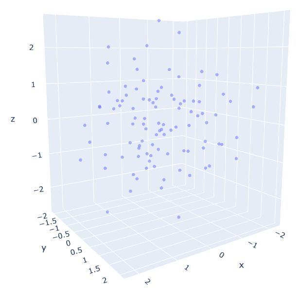
Figure 1. Data with 3D
stack = np.stack([x,y,z])
print("Shape after stacking: ",stack.shape)
print("Shape after transposing: ", stack.T.shape)
Shape after stacking:  (3, 100)
Shape after transposing:  (100, 3)
Covariance Matrix
I compute the covariance of two variables \(x\) and \(y\) using the following formula:
\[{\rm Cov}(x,y) = {1\over N-1}\sum_{j=1}^N (x_j-\mu_x)(y_j-\mu_j)\]where \(\mu_x\) and \(\mu_y\) are the means for \(x\) and \(y\).
The covariance matrix via the following equation:
\[{C} = {1\over N-1}\sum_{j=1}^N (X-\bar{x})^T(X-\bar{x})\]\(\bar{x}\) is the mean vector.
from sklearn.preprocessing import StandardScaler

X_std = stack.T

N = X_std.shape[0]

mean_vec = np.mean(X_std, axis = 0)
cov_mat = (X_std - mean_vec).T.dot((X_std - mean_vec)) / (N-1)

print("Mean vector: ")
print(mean_vec)
print()
print("Cov Matrix: ")
print(cov_mat)
Mean vector:
[-9.76996262e-17  1.03111963e-16  1.17683641e-16]

Cov Matrix:
[[ 1.01010101 -0.02569347 -0.01388866]
 [-0.02569347  1.01010101 -0.02001288]
 [-0.01388866 -0.02001288  1.01010101]]
Instead of using the above code, we could compute the covariance matrix with one line of code below.
cov_mat = np.cov(X_std.T)

print("Cov Matrix using numpy: ")
print(cov_mat)
Cov Matrix using numpy:
[[ 1.01010101 -0.02569347 -0.01388866]
 [-0.02569347  1.01010101 -0.02001288]
 [-0.01388866 -0.02001288  1.01010101]]
Eigenvectors and Eigenvalues
Eigen-decomposition of the covariance matrix is an important part of PCA. The eigenvectors are principal components determining the direction of the subspace, while the eigenvalues determine their magnitude.
Given \(A\) be a square matrix, \(ν\) a vector (eigenvector), and \(λ\) a scalar value called “eigenvalue” that satisfies \(Aν = λν\). The eigenvector of a matrix \(A\) is the vector satisfying the equation:
\[Aν = λν\] \[=> det(A-λI)=0\]where \(I\) is the identity matrix.
Using the in-built np.linalg.eig function from numpy to compute the eigenvalues and the eigenvectors of a square matrix.
eig_vals, eig_vecs = np.linalg.eig(cov_mat)

print("Eigenvectors (Lambda) \n", eig_vecs)
print("\nEigenvalues \n", eig_vals)
Eigenvectors (Lambda)
 [[ 0.58153526  0.59357932 -0.55630957]
 [ 0.62948887 -0.76149803 -0.15448145]
 [ 0.51532563  0.26035427  0.81648953]]

Eigenvalues
 [0.96998146 1.03697114 1.02335043]
I visualize 3 components which are three eigenvectors calculated above.
# Re-plot data
fig = go.Figure(data=[go.Scatter3d(x=x, y=y, z=z, mode='markers', marker=dict(size=3, opacity=0.5), name='data')])
t = np.linspace(0,1)
i=0

for idx, v in enumerate(eig_vecs.T):
    ex, ey, ez = t*v[0], t*v[1],  t*v[2]
    fig.add_trace(go.Scatter3d(x=ex, y=ey, z=ez,mode='markers', marker=dict(size=3,opacity=0.8), name="eig_vec_"+str(idx)))
fig.show()
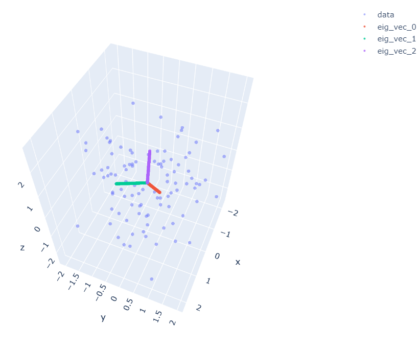
Figure 2.Three eigenvectors
Ordering and Choosing
Firstly, I sort the eigenvectors by decreasing the order of eigenvalues. Then I choose first-\(k\) columns of eigenvector matrix (where \(k\) is the number of dimensions that you want to reduce). The eigenvectors with higher eigenvalues hold much information, so the set of axes with the most information holds the most important features in the new space.
idx = eig_vals.argsort()[::-1] # Sort descending and get sorted indices
v = eig_vals[idx] # Use indices on eigv vector
w = eig_vecs[:,idx]

# keep all the eigenvectors
k=3
w[:, :k]
array([[ 0.59357932, -0.55630957,  0.58153526],
       [-0.76149803, -0.15448145,  0.62948887],
       [ 0.26035427,  0.81648953,  0.51532563]])
Projection
Finally, I transform data onto the new subspace by the dot product of data and the first \(k\) columns of eigenvector matrix. The equation:
\[y = W^T \times x\]# keep all data
k=3
new_data_all = X_std.dot(w[:,:k]) # project all data
print("Shape: ",new_data_all.shape)
print("Covariance matrix: \n",np.cov(new_data_all.T) )
print()
k=2
new_data_proj = X_std.dot(w[:,:k]) # project onto 2-D data
print("Shape: ",new_data_proj.shape)
print("Covariance matrix: \n",np.cov(new_data_proj.T) )
Shape:  (100, 3)
Covariance matrix:
 [[ 1.03697114e+00  8.44488235e-15 -3.27178770e-15]
 [ 8.44488235e-15  1.02335043e+00  4.28247619e-15]
 [-3.27178770e-15  4.28247619e-15  9.69981462e-01]]

Shape:  (100, 2)
Covariance matrix:
 [[1.03697114e+00 8.44488235e-15]
 [8.44488235e-15 1.02335043e+00]]
fig = go.Figure(data=[(go.Scatter3d(x=new_data_all[:,0], y=new_data_all[:,1], z=new_data_all[:,2],\
mode='markers', marker=dict(size=3, opacity=0.5), name="original point"))])

fig.add_trace(go.Scatter3d(x=new_data_proj[:,0], y=new_data_proj[:,1], z=new_data_proj[:,1]*0,\
mode='markers', marker=dict(size=3, opacity=0.5), name="new point"))

fig.show()
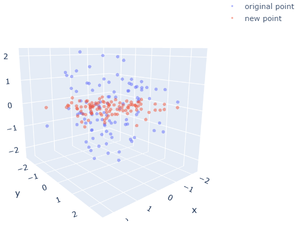
Figure 3. New subspace
Testing
I encapsulate all into a class (MyPCA) and compare the result with PCA of sklearn by visualizing on 2-D space.
import numpy as np

class MyPCA:

    def __init__(self, n_components):
        self.n_components = int(n_components)

    def __standardize(self,X):
        # standardize: z = x-mu/sigma
        self.mu = np.mean(X.T)
        self.sigma = np.std(X.T)
        X_std = (X - self.mu) / self.sigma
        return X_std

    def fit(self, X):
        #centerize data
        X -=np.mean(X.T)

        X_std = self.__standardize(X)

        cov_mat = np.cov(X_std.T)

        # decomposition
        self.eig_vals, self.eig_vecs = np.linalg.eig(cov_mat)

        #sort and choose the largest eig
        idx = self.eig_vals.argsort()[::-1]
        v = self.eig_vals[idx]
        W = self.eig_vecs[:,idx]

        self.components = W[:, :self.n_components]

        return self

    def transform(self, X):
        X_std = (X - self.mu) / self.sigma
        X_pca = np.dot(X_std,self.components)

        return np.round(X_pca, 8)

    def fit_transform(self, X, y=None):
        return self.fit(X).transform(X)

        return self.transform(X)
from sklearn.decomposition import PCA


dim = 3
N = 100

data, label = make_blobs(n_samples=N, n_features=3, random_state=2021, center_box=(-1,1), centers=None)
data = StandardScaler().fit_transform(data)

n_components = 2

my_pca = MyPCA(n_components).fit_transform(data)
pca = PCA(n_components).fit_transform(data)
plt.scatter(my_pca[:, 0], my_pca[:, 1], c='r',alpha=0.5)
plt.scatter(pca[:, 0], pca[:, 1], c='b',alpha=0.6)
plt.xlabel('component 1')
plt.ylabel('component 2')
plt.show()
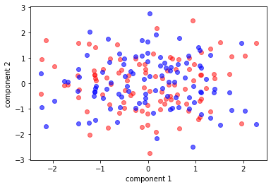
Figure 4. The red is MyPCA, The blue is PCA-sklearn
fig = go.Figure(data=[(go.Scatter3d(x=my_pca[:,0], y=my_pca[:,1], z=my_pca[:,1]*0, mode='markers', marker=dict(size=5, opacity=0.5), name="my pca"))])
fig.add_trace(go.Scatter3d(x=pca[:,0], y=pca[:,1], z=pca[:,1]*0, mode='markers', marker=dict(size=5, opacity=0.5), name="sklearn"))
fig.show()
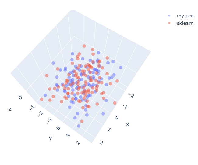
Figure 5. MyPCA has the opposite sign of PCA-sklearn
It seems MyPCA has the opposite sign of PCA-sklearn. However, the result is still right as long as each component is chosen that has the maximum amount of variance in the data. Now, we’re checking result.
x_diff = np.abs(pca[:,0]-my_pca[:,0])
print("Differnt x-axis:\n", np.max(x_diff))
y_diff = np.abs(pca[:,1]-my_pca[:,1])
print("Differnt y-axis:\n", np.max(y_diff))
Differnt x-axis:
 4.953084720149548e-09
Differnt y-axis:
 5.50720865662976
print("sklearn-PCA:\n",pca[:,1])
print()
print("My PCA:\n",my_pca[:,1])
sklearn-PCA:
 [ 0.28541527  0.63504679 -0.11113    -0.35086303 -0.31474195  0.40524636
  0.80073826  1.12177067  0.69474858 -0.56977603 -1.54261646  0.24987603
 -0.74307869 -0.18836204 -0.99361077 -0.98975223 -1.08557177  1.93069021
  1.11613657  0.21577154 -0.76230362 -0.9649021  -0.50872739 -0.32445743
  0.60136003 -0.19414276  2.75360433  0.29148234  2.03979766  0.55925086
  1.59412355  0.06689331 -1.21917872  0.7027721   0.03150815 -0.97492906
  0.49602014 -0.54554506 -1.60383125 -0.5241716   1.02700966  0.06725965
  0.05508722  1.05897591 -0.35475756 -0.41197166 -0.33981429  0.80185973
  0.07885666 -1.43432019  1.19998883 -0.20892116 -2.16947463  1.71305061
 -0.3449316  -1.62978541 -0.42120797  0.75459957 -0.95522983 -1.5910599
  0.46880642 -0.95734758 -1.69516004  1.17685374 -0.76411883  0.61849032
 -1.36233429 -0.10336255  0.83969854 -0.21238108  0.31983219 -2.4926453
  1.09182019 -0.5720852   1.63995228  1.08925999  0.16925006  0.43910527
  1.42978581  0.39215733 -0.68214688 -1.06017667 -0.94688568 -0.49442943
 -0.30530306  0.74982636  1.78349152 -1.56507263  1.74885014  1.32316246
 -0.11277267 -0.34767398 -1.02782385  0.18154674 -0.2871763   0.98239112
  0.45566674 -0.56253294 -1.17920734  0.85491462]

My PCA:
 [-0.28541527 -0.63504679  0.11113     0.35086303  0.31474195 -0.40524636
 -0.80073826 -1.12177067 -0.69474858  0.56977603  1.54261646 -0.24987603
  0.74307869  0.18836204  0.99361077  0.98975223  1.08557177 -1.93069021
 -1.11613657 -0.21577154  0.76230362  0.9649021   0.50872739  0.32445743
 -0.60136003  0.19414276 -2.75360433 -0.29148234 -2.03979766 -0.55925086
 -1.59412355 -0.06689331  1.21917872 -0.7027721  -0.03150815  0.97492906
 -0.49602014  0.54554506  1.60383125  0.5241716  -1.02700966 -0.06725965
 -0.05508722 -1.05897591  0.35475756  0.41197166  0.33981429 -0.80185973
 -0.07885666  1.43432019 -1.19998883  0.20892116  2.16947463 -1.71305061
  0.3449316   1.62978541  0.42120797 -0.75459957  0.95522983  1.5910599
 -0.46880642  0.95734758  1.69516004 -1.17685374  0.76411883 -0.61849032
  1.36233429  0.10336255 -0.83969854  0.21238108 -0.31983219  2.4926453
 -1.09182019  0.5720852  -1.63995228 -1.08925999 -0.16925006 -0.43910527
 -1.42978581 -0.39215733  0.68214688  1.06017667  0.94688568  0.49442943
  0.30530306 -0.74982636 -1.78349152  1.56507263 -1.74885014 -1.32316246
  0.11277267  0.34767398  1.02782385 -0.18154674  0.2871763  -0.98239112
 -0.45566674  0.56253294  1.17920734 -0.85491462]
flipping sign at y-axis
print("Flipping:\n",-my_pca[:,1])
Flipping:
 [ 0.28541527  0.63504679 -0.11113    -0.35086303 -0.31474195  0.40524636
  0.80073826  1.12177067  0.69474858 -0.56977603 -1.54261646  0.24987603
 -0.74307869 -0.18836204 -0.99361077 -0.98975223 -1.08557177  1.93069021
  1.11613657  0.21577154 -0.76230362 -0.9649021  -0.50872739 -0.32445743
  0.60136003 -0.19414276  2.75360433  0.29148234  2.03979766  0.55925086
  1.59412355  0.06689331 -1.21917872  0.7027721   0.03150815 -0.97492906
  0.49602014 -0.54554506 -1.60383125 -0.5241716   1.02700966  0.06725965
  0.05508722  1.05897591 -0.35475756 -0.41197166 -0.33981429  0.80185973
  0.07885666 -1.43432019  1.19998883 -0.20892116 -2.16947463  1.71305061
 -0.3449316  -1.62978541 -0.42120797  0.75459957 -0.95522983 -1.5910599
  0.46880642 -0.95734758 -1.69516004  1.17685374 -0.76411883  0.61849032
 -1.36233429 -0.10336255  0.83969854 -0.21238108  0.31983219 -2.4926453
  1.09182019 -0.5720852   1.63995228  1.08925999  0.16925006  0.43910527
  1.42978581  0.39215733 -0.68214688 -1.06017667 -0.94688568 -0.49442943
 -0.30530306  0.74982636  1.78349152 -1.56507263  1.74885014  1.32316246
 -0.11277267 -0.34767398 -1.02782385  0.18154674 -0.2871763   0.98239112
  0.45566674 -0.56253294 -1.17920734  0.85491462]
y_diff = np.abs(pca[:,1]+my_pca[:,1])
print("Differnt y-axis after flipping:\n", np.max(y_diff))
Differnt y-axis after flipping:
 4.999092251267712e-09
fig = go.Figure(data=[(go.Scatter3d(x=my_pca[:,0], y=-my_pca[:,1], z=my_pca[:,1]*0, mode='markers',\
marker=dict(size=5, opacity=0.7), name="my pca after sign-flipping"))])

fig.add_trace(go.Scatter3d(x=pca[:,0], y=pca[:,1], z=pca[:,1]*0, mode='markers', marker=dict(size=5, opacity=0.5), name="sklearn"))
fig.show()
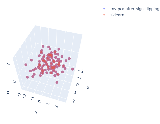
Figure 6. The result after flipping sign
fig = go.Figure(data=[(go.Scatter(x=my_pca[:,0], y=-my_pca[:,1], mode='markers',\
marker=dict(size=10, opacity=0.7), name="my pca after sign-flipping"))])

fig.add_trace(go.Scatter(x=pca[:,0], y=pca[:,1], mode='markers', marker=dict(size=10, opacity=0.5), name="sklearn"))
fig.show()
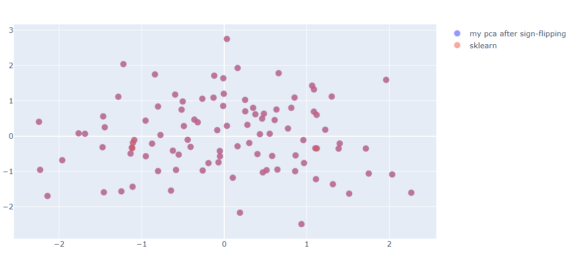
Figure 7. The result after flipping sign
After the flipping sign, The result of PCA is the same as sklearn. This notebook can be downloaded here [3].
And that’s all, hope this was interesting.
References
[1] Principal Component Analysis
[2] Why do need to normalize data before PCA