ARIMA Model - Time Series Analysis Part 1
data python timeseriesTime series is a sequence of observations collected at ordered time intervals. Time series analysis is used for many applications such as traffic prediction, sales forecasting, stock market analysis, etc bringing considerable commercial significance since then driving business plan. This i s a series of post which we’ll analyze time series data, and apply several time series models to predict bitcoin price. In the first post of this series, we walk you through the process of applying ARIMA model in Python.
ARIMA is a widely used time series forecasting that a given time series based on its own past value is used to forecast the future.
The section of the post will be organized following: In the first section, we introduce an overview of ARIMA. Subsequently, we visualize time series, and handle missing value. Next, we split data and determine the stationarity of data. We then show how to find parameters automatically. Eventually, we predict future values.
- The dataset is available here [Online accessed Jan 04 2021] [1]
- You can download this notebook here [2]. Now, let’s get started.
Contents
ARIMA Model
ARIMA stands for ‘Auto Regressive Integrated Moving Average’ used for statistical analysis of the time series data. The basic idea of the model is information in the past values of the time series can be used to predict the future values as a linear combination of its own past values, past errors, and current and past values of other time series. An ARIMA model is typically expressed as three terms p, d, and q defined as \(ARIMA(p,d,q)\) where:
- \(p\) (AR - Auto regressive) means the number of prior or lagged Y values that have to be added/subtracted to be used as predictor. In other words, it predicts future values based on past values.
- \(d\) (I - Integrated) is the number of nonseasonal differences to produce a stationary data. If \(d=0\), our data is stationary (not tend to go up or down in the long term)
- \(q\) (MA - Moving Average) is the size of moving average window. In other words, it is the number of prior or lagged values for the residual error (residual error is the difference between observed value and the corresponding fitted value) that are added/subtracted to Y.
The formual itself:
\[\begin{equation} y'_{t} = c + \phi_{1}y'_{t-1} + \cdots + \phi_{p}y'_{t-p} + \theta_{1}\varepsilon_{t-1} + \cdots + \theta_{q}\varepsilon_{t-q} + \varepsilon_{t} \end{equation}\]where:
- \(y'_{t}\) is the differenced series (it may have been differenced more than once) at time point \(t\).
- \(\phi\) and \(\theta\) are the parameters for the AR and MA components of the model respectively.
- \(\varepsilon\) is an error term.
- \(c\) is a constant.
In order to interpret the model in words:
Predicted Yt = Constant + Linear combination Lags of Y + Linear Combination of Lagged forecast errors
The goal is to identify the values of p, d and q. If you would like dive into principles of forecasting, the textbook Forecasting: Principles and Practice [3] may be useful to you.
Implementation
EDA & Preprocessing
import pandas as pd
import numpy as np

import matplotlib.pyplot as plt
import plotly.graph_objects as go


data = pd.read_csv('bitstampUSD_1-min_data_2012-01-01_to_2020-12-31.csv')
data
| Timestamp | Open | High | Low | Close | Volume_(BTC) | Volume_(Currency) | Weighted_Price | |
|---|---|---|---|---|---|---|---|---|
| 0 | 1325317920 | 4.39 | 4.39 | 4.39 | 4.39 | 0.455581 | 2.0 | 4.39 |
| 1 | 1325317980 | NaN | NaN | NaN | NaN | NaN | NaN | NaN |
| 2 | 1325318040 | NaN | NaN | NaN | NaN | NaN | NaN | NaN |
| 3 | 1325318100 | NaN | NaN | NaN | NaN | NaN | NaN | NaN |
| 4 | 1325318160 | NaN | NaN | NaN | NaN | NaN | NaN | NaN |
| ... | ... | ... | ... | ... | ... | ... | ... | ... |
| 4727774 | 1609372680 | 28850.49 | 28900.52 | 28850.49 | 28882.82 | 2.466590 | 71232.784464 | 28879.056266 |
| 4727775 | 1609372740 | 28910.54 | 28911.52 | 28867.60 | 28881.30 | 7.332773 | 211870.912660 | 28893.695831 |
| 4727776 | 1609372800 | 28893.21 | 28928.49 | 28893.21 | 28928.49 | 5.757679 | 166449.709320 | 28909.166061 |
The dataset includes 8 attributes which collected from 31 December 2011 to 31 December 2020. In this post, we only focus on 2 attributes: timestamp and weighted price. There are a lot of null values in the data. Now, our data must be preprocessed a little bit before continuing. First, We need to parse timestamp column to the second unit. Since the data is collected every one hour, we resample it by day. All time intervals in a day are averaged.
#parse datetime format

data['Timestamp'] = pd.to_datetime(data['Timestamp'], unit='s')
data = data.set_index('Timestamp')[['Weighted_Price']]
data
| Weighted_Price | |
|---|---|
| Timestamp | |
| 2011-12-31 07:52:00 | 4.390000 |
| 2011-12-31 07:53:00 | NaN |
| 2011-12-31 07:54:00 | NaN |
| 2011-12-31 07:55:00 | NaN |
| 2011-12-31 07:56:00 | NaN |
| ... | ... |
| 2020-12-30 23:56:00 | 28806.429798 |
| 2020-12-30 23:57:00 | 28846.441863 |
| 2020-12-30 23:58:00 | 28879.056266 |
| 2020-12-30 23:59:00 | 28893.695831 |
| 2020-12-31 00:00:00 | 28909.166061 |
#resample by day

daily_data = data.resample("D").mean()
daily_data
| Weighted_Price | |
|---|---|
| Timestamp | |
| 2011-12-31 | 4.471603 |
| 2012-01-01 | 4.806667 |
| 2012-01-02 | 5.000000 |
| 2012-01-03 | 5.252500 |
| 2012-01-04 | 5.208159 |
| ... | ... |
| 2020-12-27 | 27043.386470 |
| 2020-12-28 | 26964.020499 |
| 2020-12-29 | 26671.008099 |
| 2020-12-30 | 28141.234408 |
| 2020-12-31 | 28909.166061 |
fig = go.Figure()
fig.add_trace(go.Scatter(x=daily_data.index, y=daily_data['Weighted_Price'], name='Weighted Price'))
fig.update_layout(title="BTC price history", xaxis_title="Datetime", yaxis_title="Weighted Price")
fig.show()

btc_data = daily_data.copy()[['Weighted_Price']]
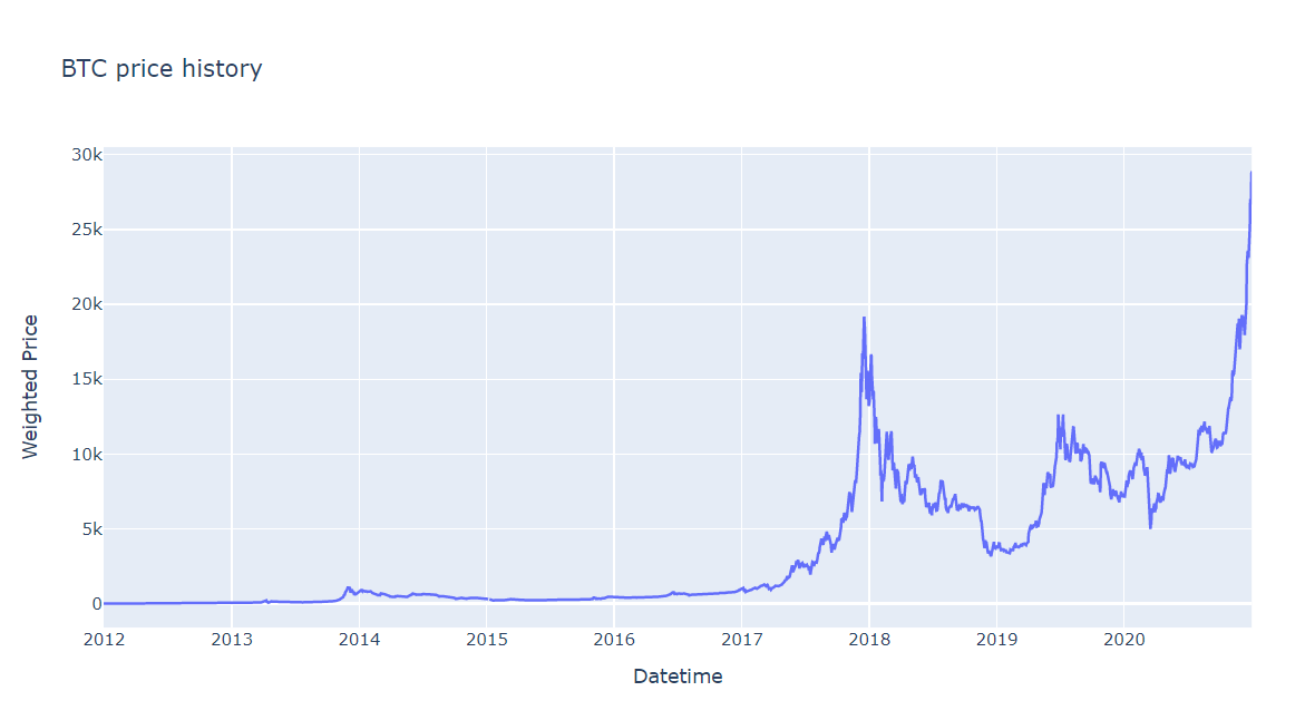
Figure 1. Data Visualization
Let’s plot the whole scene. Next, we need to check null in data. If data exists null values, we’ll process them.
print("N null: ",btc_data.isnull().sum())
N null:  Weighted_Price    3
dtype: int64
There are 3 null values in the data, we fill in them by averaging between the previous 3 points and the next 3 points at the null position.
arr_null = np.where(btc_data.isnull()==True)[0]
print("Index of null: ", arr_null)

if np.where(btc_data.isnull()==True):
    val_fill_null = btc_data[min(arr_null)-3:max(arr_null)+4].mean()[0]
    btc_data = btc_data.fillna(val_fill_null,inplace = False)
Index of null: [1102 1103 1104]
Data Splitting & Augmented Dickey-Fuller test
After preprocessing data, we start building the model. The first process is to split data. We create training set in 7 years, the rest is test set (from early 2019 to late 2020).
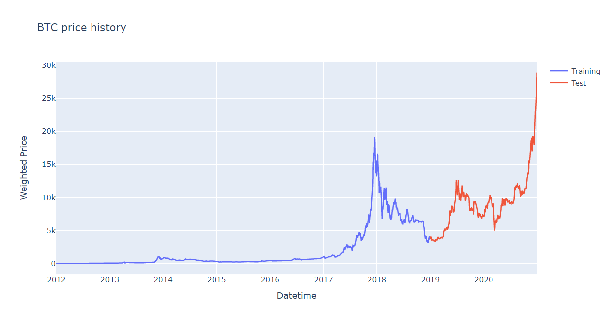
Figure 2. Data Splitting
Next, we determine our time series is stationary. It means the mean and variance are constant over time. In other words, time series does not have a trend (not go up or down over time). This makes the model easier to predict.
We can use the Augmented Dickey-Fuller (ADF) test, in which the null hypothesis of the test is non-stationary series. So, if the p-value of the test is less than 0.05, we reject the null hypothesis and infer that the time series is stationary.
from statsmodels.tsa.stattools import adfuller

result = adfuller(train_data)

print('ADF Statistic: %f' % result[0])
print('p-value: %f' % result[1])
print('Critical Values:')
for key, value in result[4].items():
    print('\t%s: %.3f' % (key, value))
ADF Statistic: -1.891007
p-value: 0.336303
Critical Values:
	1%: -3.433
	5%: -2.863
	10%: -2.567
The p-value is greater than 0.05 (0.3363), the time series is non-stationary. To make series is stationary, we will need to difference the data until we obtain a stationary time series. In this step, we can determine \(p\) paramater in ARIMA.
When you only remove the previous Y values only once, it is called “first-order difference”. Mathematically:
\[y_{t} = y_t - y_{t-1}\]first_diff = train_data.diff()
result = adfuller(first_diff[1:])
print('ADF Statistic: %f' % result[0])
print('p-value: %f' % result[1])
print('Critical Values:')
for key, value in result[4].items():
print('\t%s: %.3f' % (key, value))
ADF Statistic: -9.355544
p-value: 0.000000
Critical Values:
	1%: -3.433
	5%: -2.863
	10%: -2.567
After 1 time differencing, the p-value is 0.000000 less than 0.05 and we set the order of differencing \(d = 1\). \(p\) and \(q\) terms will be find automatically in the next section.
Fitting and Forecasting
The pmdarima package is used to find the appropriate ARIMA model. auto_arima will find \(p\) and \(q\) automatically based AIC measure.
import pmdarima as pm

auto = pm.auto_arima(
    train_data, d=1,
    seasonal=False, stepwise=True,
    suppress_warnings=True, error_action="ignore",
    max_p=6, max_order=None, trace=True
)

auto.plot_diagnostics(figsize=(9,6))
plt.show()
Performing stepwise search to minimize aic
 ARIMA(2,1,2)(0,0,0)[0] intercept   : AIC=33445.437, Time=1.31 sec
 ARIMA(0,1,0)(0,0,0)[0] intercept   : AIC=33572.801, Time=0.04 sec
 ARIMA(1,1,0)(0,0,0)[0] intercept   : AIC=33482.242, Time=0.09 sec
 ARIMA(0,1,1)(0,0,0)[0] intercept   : AIC=33492.166, Time=0.13 sec
 ARIMA(0,1,0)(0,0,0)[0]             : AIC=33570.980, Time=0.03 sec
 ARIMA(1,1,2)(0,0,0)[0] intercept   : AIC=33444.809, Time=1.19 sec
 ARIMA(0,1,2)(0,0,0)[0] intercept   : AIC=33475.869, Time=0.20 sec
 ARIMA(1,1,1)(0,0,0)[0] intercept   : AIC=33482.449, Time=0.30 sec
 ARIMA(1,1,3)(0,0,0)[0] intercept   : AIC=33445.568, Time=1.44 sec
 ARIMA(0,1,3)(0,0,0)[0] intercept   : AIC=33473.566, Time=0.33 sec
 ARIMA(2,1,1)(0,0,0)[0] intercept   : AIC=33445.143, Time=1.69 sec
 ARIMA(2,1,3)(0,0,0)[0] intercept   : AIC=33446.062, Time=3.13 sec
 ARIMA(1,1,2)(0,0,0)[0]             : AIC=33442.902, Time=0.63 sec
 ARIMA(0,1,2)(0,0,0)[0]             : AIC=33473.978, Time=0.12 sec
 ARIMA(1,1,1)(0,0,0)[0]             : AIC=33480.563, Time=0.18 sec
 ARIMA(2,1,2)(0,0,0)[0]             : AIC=33443.531, Time=0.70 sec
 ARIMA(1,1,3)(0,0,0)[0]             : AIC=33443.658, Time=0.76 sec
 ARIMA(0,1,1)(0,0,0)[0]             : AIC=33490.299, Time=0.06 sec
 ARIMA(0,1,3)(0,0,0)[0]             : AIC=33471.687, Time=0.13 sec
 ARIMA(2,1,1)(0,0,0)[0]             : AIC=33443.257, Time=0.56 sec
 ARIMA(2,1,3)(0,0,0)[0]             : AIC=33444.160, Time=0.98 sec

Best model:  ARIMA(1,1,2)(0,0,0)[0]
Total fit time: 14.008 seconds
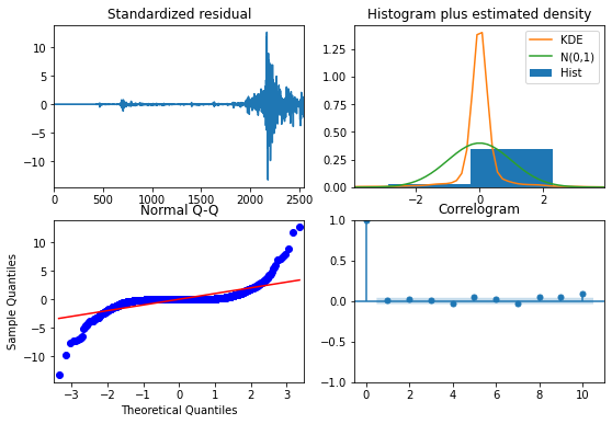
Figure 3. Model diagnostics
The output of our code recommends \(ARIMA(1,1,2)\) is the best model when yielding the lowest AIC value of 33442.90. After using grid search, we have determined the full set of parameters. Now, we use these parameters to feed into ARIMA (statsmodels package).
import warnings
warnings.filterwarnings('ignore')

from statsmodels.tsa.arima_model import ARIMA


mod = ARIMA(train_data, order=(1,1,2))
results = mod.fit(disp=0)
print(results.summary())
                             ARIMA Model Results
==============================================================================
Dep. Variable:       D.Weighted_Price   No. Observations:                 2554
Model:                 ARIMA(1, 1, 2)   Log Likelihood              -16717.389
Method:                       css-mle   S.D. of innovations            168.444
Date:                Sat, 15 May 2021   AIC                          33444.777
Time:                        14:52:48   BIC                          33474.004
Sample:                    01-01-2012   HQIC                         33455.376
                         - 12-28-2018
==========================================================================================
                             coef    std err          z      P>|z|      [0.025      0.975]
------------------------------------------------------------------------------------------
const                      1.4443      4.055      0.356      0.722      -6.503       9.392
ar.L1.D.Weighted_Price    -0.9310      0.024    -38.834      0.000      -0.978      -0.884
ma.L1.D.Weighted_Price     1.1252      0.030     37.988      0.000       1.067       1.183
ma.L2.D.Weighted_Price     0.2241      0.019     11.744      0.000       0.187       0.261
                                    Roots
=============================================================================
                  Real          Imaginary           Modulus         Frequency
-----------------------------------------------------------------------------
AR.1           -1.0741           +0.0000j            1.0741            0.5000
MA.1           -1.1540           +0.0000j            1.1540            0.5000
MA.2           -3.8670           +0.0000j            3.8670            0.5000
-----------------------------------------------------------------------------
We predict in history data after fitting model, it looks like good fit.
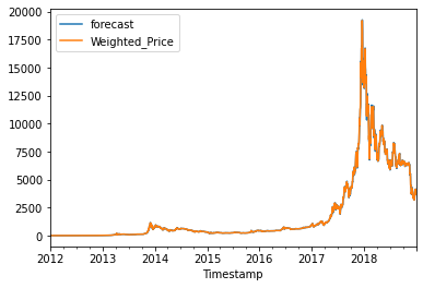
Figure 4. Predicting history data
Although ARIMA performs well in history data, it forecasts the bad result in the futre. When we conduct a forecast in test set, the forecast line is just a straight line. This is not what we expect in the forecast.
n_period=test_data.shape[0]
fc, se, conf = results.forecast(n_period)

# Make as pandas series
fc_series = pd.Series(fc, index=test_data.index[:n_period])
lower_series = pd.Series(conf[:, 0], index=test_data.index[:n_period])
upper_series = pd.Series(conf[:, 1], index=test_data.index[:n_period])

# Plot
plt.figure(figsize=(12,5), dpi=100)
plt.plot(train_data, label='training')
plt.plot(test_data[:n_period], label='actual')
plt.plot(fc_series, label='forecast')
plt.fill_between(lower_series.index, lower_series, upper_series,
                 color='k', alpha=.15)
plt.title('Forecast vs Actuals')
plt.legend(loc='upper left', fontsize=8)
plt.show()
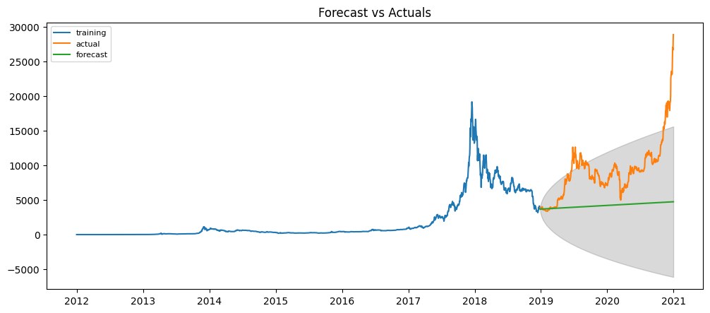
Figure 5. ARIMA prediction
y_truth = test_data['Weighted_Price'].values
y_forecasted = forecast
mse_arima = ((y_forecasted - y_truth) ** 2).mean()
print('The Mean Squared Error of ARIMA: {}'.format(mse_arima)
The Mean Squared Error of ARIMA: 39110912.718644276
We need to improve to get better. In the time series model, the predictions over time become less and less accurate. To overcome this problem, walk-forward validation is the most preferred solution. In walk-forward validation, we take few steps back in time and forecast the future as many steps you took back. Then you compare the forecast against the actuals.
test_arima = test_data.copy()
train_arima = train_data.copy()

history = [x for x in train_arima.values]
predictions = list()

# walk-forward validation
for t in range(test_arima.shape[0]):
    model = ARIMA(history, order=(1,1,2))
    arima_results = model.fit()

    output = arima_results.forecast()
    yhat = output[0]
    predictions.append(yhat)

    obs = test_arima.iloc[t].values

    #append forecast value into history data
    history.append(obs)

predictions = np.array(predictions)
test_arima['y_pred'] = predictions
y_forecasted = test_arima['y_pred'].values
y_truth = test_arima['Weighted_Price'].values

# Compute the mean square error
mse_arima = ((y_forecasted - y_truth) ** 2).mean()
print('The Mean Squared Error of ARIMA is {}'.format(mse_arima))
The Mean Squared Error of ARIMA is 83972.33422899031
fig = go.Figure()
fig.add_trace(go.Scatter(x=test_arima.index, y=test_arima['Weighted_Price'], name='Actual'))
fig.add_trace(go.Scatter(x=test_arima.index, y=test_arima['y_pred'], name='Forecast'))
fig.update_layout(title="BTC - Forecast", xaxis_title="Datetime", yaxis_title="Weighted Price")
fig.show()
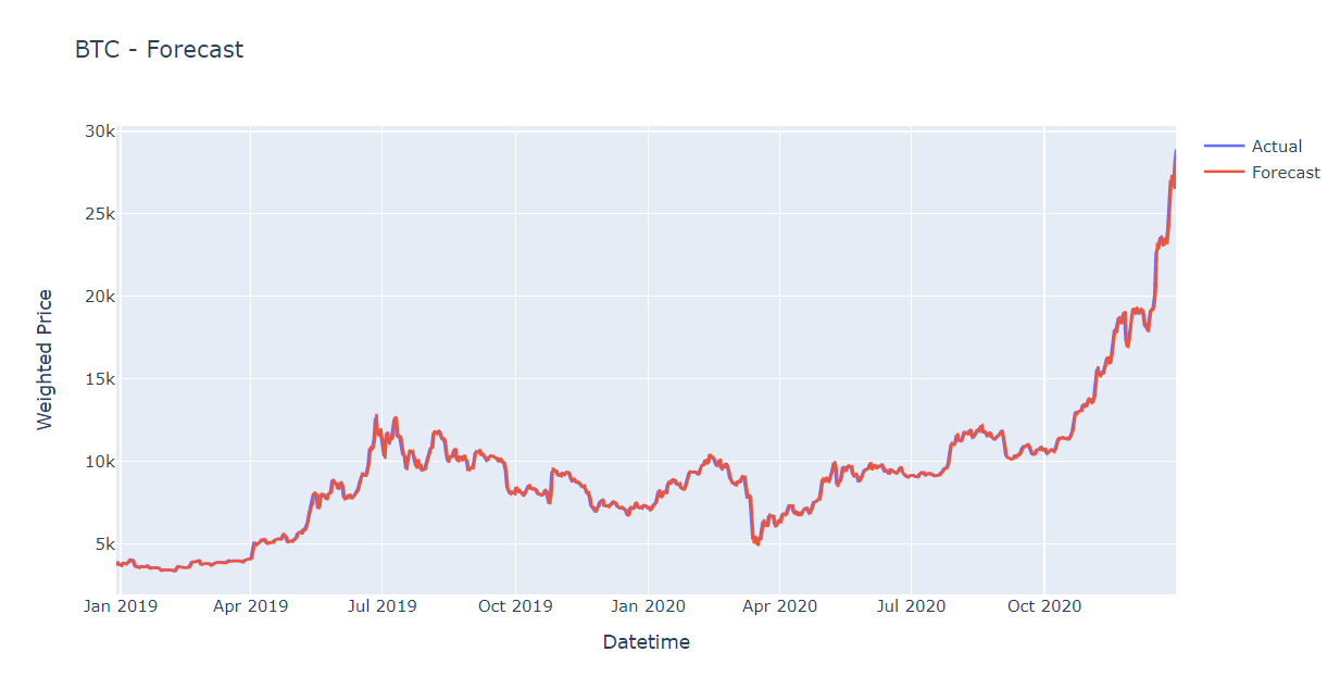
Figure 6. ARIMA prediction with walk-forward validation
The forecast line becomes better when we apply the walk-forward validation technique. Intuitively, we feel that’s good, however, the mean squared error is still very high that needs improving.
Conclusion
In this tutorial, we describe how to implement ARIMA model for univariate time series forecasting in Python. In the following posts, we try to cover a lot of other models and improve the results.
Hope that this post was helpful for you.
References
[1] Bitcoin Historical Data [Online accessed Jan 04 2021]